Recurrence relations and linear algebra

I recently learned that GitHub markdown doesn’t have native support for rendenring math equations. That seemed quite weird, so I figured that I’d try to look at existing alternatives and flex my tex muscle.

In this post I will try to show an end-to-end example of how to solve linear ordinary recurrence relations and give an intro to all the linear algebra required to do that. Some basic understanding of vector spaces and matrices is still required though.

Fibonacci sequence

And of course I will start with a well known example of Fibonacci sequence defined as follows:

\[F_n = \begin{cases} F_{n - 1} + F_{n - 2}, & \text{if $n \ge 2$} \\ 1, & \text{if $n = 1$} \\ 0, & \text{if $n = 0$} \end{cases}\]

Here are the first few elements of the sequence:

\[0, 1, 1, 2, 3, 5, 8, \ldots\]

The Fibonacci sequence is well known and well studies, so it’s hardly worth spending much time on introducing it. Moreover in this post I will not find anything new about this sequence, but I will show how we could derive a non-recurrent formula for the nth member of the sequences or, in other words, how to solve this kind of recurrence.

Matrix form

The first step would be to rewrite the same recurence relation in a matrix form. The goal is to find a matrix A such that the following equation holds:

\[\begin{bmatrix} F_{n} \\ F_{n-1} \end{bmatrix} = A \begin{bmatrix} F_{n - 1} \\ F_{n - 2} \end{bmatrix}\]

It’s not hard to see that the following matrix satisfies the conditions:

\[\begin{bmatrix} F_{n} \\ F_{n-1} \end{bmatrix} = \begin{bmatrix} 1 & 1 \\ 1 & 0 \\ \end{bmatrix} \begin{bmatrix} F_{n - 1} \\ F_{n - 2} \end{bmatrix}\]

We can easily do that because the Fibonacci recurrence relation is linear. In general for linear recurrence relations the size of the matrix and vectors involved in the matrix form will be identied by the order of the relation.

In case of the Fibonacci sequence, with exception of the first two elements, all other elements of the sequence depend on two previous elements.

What about the first two elements of the sequence though? They serve as initial conditions for the recurrence relation, so let’s try to add them into our matrix form. In order to do that let’s expand the vector in the right side of the equation:

\[\begin{bmatrix} F_{n} \\ F_{n-1} \end{bmatrix} = A \begin{bmatrix} F_{n - 1} \\ F_{n - 2} \end{bmatrix} = A A \begin{bmatrix} F_{n - 2} \\ F_{n - 3} \end{bmatrix} = A^2 \begin{bmatrix} F_{n - 2} \\ F_{n - 3} \end{bmatrix}\]

We can continue this expnasion until we get \(F_1\) and \(F_0\), our first two members, in the right side of the equation:

\[\begin{bmatrix} F_{n} \\ F_{n-1} \end{bmatrix} = A^{n - 1} \begin{bmatrix} F_1 \\ F_0 \end{bmatrix} = A^{n-1} \begin{bmatrix} 1 \\ 0 \end{bmatrix}\]

So now we have Fibonacci sequence defined in a matrix form, does it give us anything? Conincedentally it gives us a rather cool way to calculate a Fibonacci number by given index using Exponentiation by squaring.

The algorithm takes \(O(\log n)\) matrix multiplications. Each matrix multiplication takes a fixed number of arithmetic operations on numbers, specifically 4 number multiplications and 2 number additions.

That, compared to the naive algorithm that takes \(O(n)\) additions, might seem like an improvement, especially if you assume that both multiplications and additions of integer numbers are equal constant time operations.

NOTE: Assumption that integer multiplications and additions are equal is in fact quite limiting for fast growing sequences like Fibonacci. That basically limits you to just a few dozens first members of the Fibonacci sequence that fit into machine word. If that’s a reasonable limitation for your use case, you can as well precalculate all the Fibonacci numbers you need in advance and access the in constant time when you need them. That being said with the right integer multiplication algorithm you can get an asymptotic improvement using the matrix multiplication method over the naive method.

Basises and coordinates

We now have Fibonacci recurrence relation written in the matrix form. That means that we can treat the matrix A as a linear operator in vector space \(\mathbb{R}^2\). How does it help us?

In order to see how does it help us we should talk a little bit about basises of vector spaces. More specifically, we should note that the same vector space may have multiple different basises.

For example, let’s say we have a vector t on a plane (\(\mathbb{R}^2\)) and we use x and y coordinates to describe the vector on that plane.

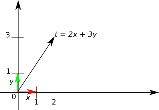
Basically x and y coordinates tell us how many basis vectors we need to combine to get the original vector t. On the picture above we need to take the vector x two time and the vector y three times, so the coordinates of the vector t in the basis consisting of vectors x and y are two and three:

\[t = \begin{bmatrix} 2 \\ 3 \end{bmatrix}\]

The pair of basis vectors chosen above is convinient to use, but that’s by no means the only pair of vectors that could be used for this purpose. For example, the two vectors u and v on this picture will work as well:

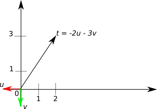
We can use those vectors as a basis as well. However the coordinates of the vector t will be different if we use them as a vector. In case of the basis consisting of vectors u and v the coordinates of the same vector t will be minus two and minus three:

\[t = \begin{bmatrix} -2 \\ -3 \end{bmatrix}\]

NOTE: you can see how it can get confusing, the same vector t in matrix notation can look completely differently depending on the basis we are working with. You might think that a good notation should specify the basis we are working with somehow, but in practice we often don’t care what the basis we are using exactly.

In this particular case if we want to switch from one basis to another all we need to do is to change the signes of coordinates to the opposite, but in general the transformation might be more complicated.

So we can have different basises for the same vector space, so what? Well, as vector coordinates look differently in different basis the matrices of linear operators might look differently in different basises. What if we can find such a basis that makes the matrix of the linear operator more convenient to work with?

Basis changes

Before we go into details regarding what matrix would be convenient to work with let’s close one purely technical question. Say we have a matrix of a linear operator in one basis, how can we convert it to represent the same linear operator but in different basis?

For a set of vectors to be a basis it’s necessary that every element of the vector space can be expressed as a linear combination of the basis vectors. That’s, of course, also true for vectors of the different basis.

In practice that means that we can find a matrix S, that given coordinates of a vector in one basis transforms them into coordinates of the same vector in another basis.

Let’s say that the original basis consits of vectors x and y and the target basis consists of vectors u and v. We know that vectors x and y can be expressed as a linear combination of vectors u and v.

Without loss of generality lets say that \(x = s_{0,0} u + s_{1,0} v\) and \(y = s_{0,1} u + s_{1,1} v\). In other words, in the basis cosisting of vectors u and v the vector x has coordinates \(s_{0,0}\) and \(s_{1,0}\), and the vector y has coordinates \(s_{0,1}\) and \(s_{1,1}\).

It’s easy to see that the matrix that converts coordinates in basis x and y to the coordinates in basis u and v will look like this:

\[S = \begin{bmatrix} s_{0,0} & s_{0,1} \\ s_{1,0} & s_{1,1} \end{bmatrix}\]

So now we can easily convert coordinates of a vector in one basis to coordinates of the same vector in another basis. How can we extend it to linear operators?

Let’s say we have a matrix A of a linear operator that works with coordinates in basis x and y. We also have a matrix S that given coordinates in basis x and y converts them to coordinates of the same vector in basis u and v.

Let’s first note that if we can convert x and y coordinates to u and v coordinates using matrix S, then we can use the inverse matrix to do the opposite transformation from u and v coordinates to x and y coordinates.

Now, if we have a vector t in u and v coordinates and we don’t know how to apply the linear transformation to it, we can first convert u and v coordinates to x and y coordinates and then apply the linear operator by multipling by the matrix A.

However that will give us a vector in x and y coordinates, but we need a vector in u and v coordinates. Well, no problem, we can just multiply it by the inverse of S to covert the vector back into the u and v coordinates.

So in order to calculate the result of linear operator in u and v coordinates we can:

1. convert the u and v coordinates to x and y coordinates using S
2. multiple by matrix A
3. convert the x and y coordinates to u and v coordinates using the inverse of S

Alternatively putting all of that in a matrix form, if A is a matrix that represents the linear operator in the basis x and y, then to apply the same transformation to a vector t with coordinates in basis u and v we can do this \(S A S^{-1} t\). Therefore the matrix that represents our linear operator in the basis u and v is \(S A S^{-1}\).

Diagonalization

So now we know how to change the matrix of a linear operator when we change from one basis to another. Now we can try to find a basis in which the matrix of our operator is simple.

What matrix is easy to work with? Let’s return back to the original problem. We had a matrix that we need to take to the power n, maybe we should look for a matrix that is easy to multiply. Diagonal matrices seem to be rather easy to multiply.

To formalize the problem we want to find a matrix B such that \(A = S B S^{-1}\) and B is diagonal. Here S is matrix that converts the coordinates from the basis where the linear operator is expressed by matrix B to the basis where the same linear operator is expressed by matrix A.

If we manage to do that, then it should be easy to get A to the power:

\[A^{n-1} = (S B S^{-1})^{n-1} = S B S^{-1} S B S^{-1} \ldots S B S^{-1} = S B^{n-1} S^{-1}\]

NOTE: it should be noted that a basis that makes B diagonal may not even exist. So we will try to find it, but no guarantees in general.

To understand how to find a basis that makes B diagonal let’s consider what the multiplication by diagonal B actually means. This multiplication will just scale each coordinate of the vector by a constant.

Remember what coordinates of the vector in a basis mean? They mean how many basis vectors we need to take to construct the original vector from them. So if a linear operator matrix is diagonal in a basis, it means that the linear operator when applied to the vectors of this basis just multiplies them by a constant. In other words it makes them longer or shorter (it can also rotate them in the opposite direction, that what multiplication by a negative value means).

So what we are looking for is a bunch of linearly independent vectors that when trasnformed by A just scale by a constant. We only care about non-trivial vectors that can constitute a basis, so the vector of length 0 is not good.

Putting it in a form of equation:

\[A x = \lambda x, \text{where} \lambda \ne 0\]

Vectors that satisfy this equation are called eigenvectors and the values of \(\lambda\) are called eigenvalues.

So if we find enough linearly independent eigenvectors, we can construct a basis in which matrix B representing the linear operator we care about is diagonal.

Finding eigenvectors

Now we need to solve the matrix equation, but it’s not a usual matrix equation because we have a parameter \(\lambda\) value of which we don’t know.

Let’s start from shuffling things around first:

\[A x = \lambda x \iff A x - \lambda x = 0\]

Now we will do an interesting manipulation: we want to extract x in the left part, but A and \(\lambda\) are matrix and a scalar and we don’t know how to substract a scalar from a matrix in general case.

However in this case we have a trick: matrix equation can be viewed as a system of linear equations. In our case A is a two by two matrix, but the same principle works in general:

\[\displaylines{ A x - \lambda x = 0 \iff \begin{bmatrix} a_{0,0} & a_{0,1} \\ a_{1,0} & a_{1,1} \end{bmatrix} \begin{bmatrix} x_0 \\ x_1 \end{bmatrix} - \begin{bmatrix} \lambda x_0 \\ \lambda x_1 \end{bmatrix} = 0 \iff \begin{cases} a_{0,0} x_0 + a_{0,1} x_1 - \lambda x_0 = 0 \\ a_{1,0} x_0 + a_{1,1} x_1 - \lambda x_1 = 0 \end{cases} \iff \begin{cases} (a_{0,0} - \lambda) x_0 + a_{0,1} x_1 = 0 \\ a_{1,0} x_0 + (a_{1,1} - \lambda) x_1 = 0 \end{cases} \iff \\ \begin{bmatrix} a_{0,0} - \lambda & a_{0,1} \\ a_{1,0} & a_{1,1} - \lambda \end{bmatrix} \begin{bmatrix} x_0 \\ x_1 \end{bmatrix} = 0 \iff (A - \lambda \mathbb{I}) x = 0 }\]

Here we use \(\mathbb{I}\) to denote a unit matrix - matrix that has ones on the main diagonal and zeros everywhere else.

Now we have a regular matrix equation with a parameter \(\lambda\). Stepping back for a second, our goal is to find enough eigenvectors to create a basis. The matrix equation above has non-trivial solutions if and only if the determinat of the matrxi \(A - \lambda \mathbb{I})\) is zero. So probably we should find such lambdas that make the determinant zero if we want to find non-trivial solutions to the equation.

In general the determinat of the two by two matrix can be calculated as follows:

\[\begin{vmatrix} a_{0,0} & a_{0,1} \\ a_{1,0} & a_{1,1} \end{vmatrix} = a_{0,0} a_{1,1} - a_{0,1} a_{1,0}\]

In case of our specific matrix we have:

\[\begin{vmatrix} 1 - \lambda & 1 \\ 1 & -\lambda \end{vmatrix} = -\lambda (1 - \lambda) - 1 = \lambda^2 - \lambda - 1\]

What is left is to solve the quadratic equation to find possible values for \(\lambda\):

\[\lambda_{0,1} = {1 \pm \sqrt{5}\over 2}\]

For convenience we will denote the solutions as follows (it’s a common notation for golden ratio and golden ratio conjugate):

\[\begin{cases} \varphi = {1 + \sqrt{5} \over 2} \\ \bar \varphi = {1 - \sqrt{5} \over 2} \end{cases}\]

So now we know two possible values of \(\lambda\), so what remains to be done is to solve the matrix equation for each value of \(\lambda\). Let’s do that:

\[\displaylines{ \begin{bmatrix} 1 - \varphi & 1 \\ 1 & -\varphi \end{bmatrix} \begin{bmatrix} x_0 \\ x_1 \end{bmatrix} = 0 \iff \begin{cases} (1 - \varphi) x_0 + x_1 = 0 \\ x_0 - \varphi x_1 = 0 \end{cases} \iff \begin{cases} (1 - \varphi) x_0 + x_1 = 0 \\ x_0 = \varphi x_1 \end{cases} \iff \begin{cases} (1 - \varphi) \varphi x_1 + x_1 = 0 \\ x_0 = \varphi x_1 \end{cases} \iff \\ \begin{cases} (-\varphi^2 + \varphi + 1) x_1 = 0 \\ x_0 = \varphi x_1 \end{cases} }\]

We have an interesting situation. You see \(\varphi\) is a root of \(\lambda^2 - \lambda + 1 = 0\) - that’s how we found it in the first place. Therefore it’s also a root of \(-\lambda^2 + \lambda - 1 = 0\), so necessarily \(-\varphi^2 + \varphi + 1 = 0\). That basically means that \(x_1\) can be literaly anything.

We are free to pick whatever value we need. Remeber that the vectors that we need must not be zero vectors, so it makes sense to pick a non-zero value for \(x_1\). Let’s pick a number that would be easy to work with, so here is our first eignevector and also our first basis vector:

\[x_0 = \begin{bmatrix} \varphi \\ 1 \end{bmatrix}\]

Repeating the same process with the \(\bar \varphi\) will give us a similar result:

\[x_1 = \begin{bmatrix} \bar \varphi \\ 1 \end{bmatrix}\]

Putting it all together

We picked a basis that is convenient and makes the matrix B of our linear operator diagonal. It’s not suprising that on the diagonal the matrix will have eigenvalues (you may want to actually verify it, but since that’s how we were looking for the eigenvalues and eigenvectors in the first place I will skip it):

\[B = \begin{bmatrix} \varphi & 0 \\ 0 & \bar \varphi \end{bmatrix}\]

The matrix that converts from the basis we found in the previous section to our original basis (we called it S in the formal problem statement above) is:

\[S = \begin{bmatrix} \varphi & \bar \varphi \\ 1 & 1 \end{bmatrix}\]

I will not show how to find the inverse of S, but you can verify that the following matrix is indeed the inverse of S:

\[S^{-1} = \begin{bmatrix} {1\over \varphi - \bar \varphi} & {- \bar \varphi \over \varphi - \bar \varphi} \\ {-1\over \varphi - \bar \varphi} & {\varphi \over \varphi - \bar \varphi} \end{bmatrix}\]

Putting it all together:

\[\displaylines{ A^n = S B^{n-1} S^{-1} = \begin{bmatrix} \varphi & \bar \varphi \\ 1 & 1 \end{bmatrix} \begin{bmatrix} \varphi & 0 \\ 0 & \bar \varphi \end{bmatrix}^{n-1} \begin{bmatrix} {1\over \varphi - \bar \varphi} & {- \bar \varphi \over \varphi - \bar \varphi} \\ {-1\over \varphi - \bar \varphi} & {\varphi \over \varphi - \bar \varphi} \end{bmatrix} = \begin{bmatrix} \varphi & \bar \varphi \\ 1 & 1 \end{bmatrix} \begin{bmatrix} \varphi^{n-1} & 0 \\ 0 & {\bar \varphi}^{n-1} \end{bmatrix} \begin{bmatrix} {1\over \varphi - \bar \varphi} & {- \bar \varphi \over \varphi - \bar \varphi} \\ {-1\over \varphi - \bar \varphi} & {\varphi \over \varphi - \bar \varphi} \end{bmatrix} = \\ {1\over \varphi - \bar \varphi} \begin{bmatrix} \varphi & \bar \varphi \\ 1 & 1 \end{bmatrix} \begin{bmatrix} \varphi^{n-1} & 0 \\ 0 & {\bar \varphi}^{n-1} \end{bmatrix} \begin{bmatrix} 1 & - \bar \varphi \\ -1 & \varphi \end{bmatrix} }\]

Now we need to multiply all those matrices. It looks hard, but we only need to do it once:

\[\displaylines{ {1\over \varphi - \bar \varphi} \begin{bmatrix} \varphi & \bar \varphi \\ 1 & 1 \end{bmatrix} \begin{bmatrix} \varphi^{n-1} & 0 \\ 0 & {\bar \varphi}^{n-1} \end{bmatrix} \begin{bmatrix} 1 & - \bar \varphi \\ -1 & \varphi \end{bmatrix} = {1\over \varphi - \bar \varphi} \begin{bmatrix} \varphi & \bar \varphi \\ 1 & 1 \end{bmatrix} \begin{bmatrix} \varphi^{n-1} & - \bar \varphi \varphi^{n-1} \\ - {\bar \varphi}^{n-1} & \varphi {\bar \varphi}^{n-1} \end{bmatrix} = \\ {1\over \varphi - \bar \varphi} \begin{bmatrix} \varphi^n - {\bar \varphi}^n & - \varphi \bar \varphi ({\bar \varphi}^{n-1} - \varphi^{n-1}) \\ \varphi^{n-1} - {\bar \varphi}^{n-1} & \varphi {\bar \varphi}^{n-1} - \bar \varphi \varphi^{n-1} \end{bmatrix} }\]

Fortunately we can stop here, as what we want to do in the end to calculate \(F_n\) is to multiply this monstrosity of a mamtrix by a rather simple vector:

\[\begin{bmatrix} F_1 \\ F_0 \end{bmatrix} = \begin{bmatrix} 1 \\ 0 \end{bmatrix}\]

Moreover we only need to take the first element of the result, which gives us a rather simple expression:

\[F_n = {\varphi^n - {\bar \varphi}^n \over \varphi - \bar \varphi} = {1\over\sqrt{5}}\left({1+\sqrt{5}\over 2}\right)^n - {1\over\sqrt{5}}\left({1-\sqrt{5}\over 2}\right)^n\]

Instead of conclusion

Hopefully it was a rather simple to understand example that ties together various parts of basic linear algebra. Of course, I skipped all the interesting stuff like proofs, but I tried to make it as intuitive as possible.